|
An Atomic Database for Spectroscopic Diagnostics of Astrophysical Plasmas
|
|
USER GUIDE - Version 8.0 - August 2015 |
|
Written by Giulio Del Zanna |
|
with contributions from P.Young, E.Landi, K.Dere, H.Mason |
Contents
1 Introduction
2 What is new in version 8
3 The CHIANTI distribution and installation
3.1 Within SolarSoft
3.2 As a stand-alone
3.3 As ChiantiPy
4 The database
5 The Software
6 Some examples on how to use the software
6.1 Calculating line intensities.
6.2 Calculating continuum intensities
6.3 Creating a synthetic spectrum with the continuum
6.4 Density and temperature diagnostics from line ratios
6.5 Looking at level populations
6.6 Looking at the different ionisation equilibria
6.7 Calculating contribution functions
6.8 Calculating radiative losses
6.9 Ionization and recombination
6.10 Electron excitation rates
1 Introduction
The CHIANTI package consists of a critically evaluated set of atomic
data, a number of ancillary data and a
suite of Interactive Data Language (IDL) programs.
CHIANTI is a collaborative project involving
the following Universities:
Cambridge (UK), George Mason and Michigan (USA).
This document is mainly intended as a quick reference to
some of the main features of CHIANTI.
Please read the CHIANTI USER GUIDE for more details and see
the main CHIANTI homepage:
http://www.chiantidatabase.org/
The CHIANTI package is freely available. We only ask you
to acknowledge and reference CHIANTI appropriately.
If a detail work on a particular ion is done,
it would be appropriate to also refer to the original publication.
References can be found at the end of each data file or on the WWW.
To keep updated on CHIANTI developments, please
read the CHIANTI pages on the WWW and
join the CHIANTI google group for comments and questions:
https://groups.google.com/forum/#!forum/chianti
2 What is new in version 8
Until now, the format of the CHIANTI files has remained the same
(aside from an update in the collisional files, to allow nine-point splines).
The changes that are introduced in version 8 are minor, in the sense that they
only affect the format of the energy and the electron excitation files.
The format of these files is different, but still fixed, i.e. the same
for all the ions.
The energy files have the same information, although the format is changed
and some redundant information has been removed.
For new ions, we have chosen not to fit the electron excitation data,
but rather to provide the original rates, still in the Burgess and Tully (1992)
scaled domain.
For each transition, a scaled temperature is given.
We have modified the IDL software that reads the new files.
There is no backward compatibility with previous versions of CHIANTI.
Finally, we have modified the DEM inversion program.
3 The CHIANTI distribution and installation
The CHIANTI database is currently distributed in three ways.
3.1 Within SolarSoft
The main CHIANTI distribution is within
SolarSoft, a programming and data analysis
environment for the solar physics community. See
http://www.lmsal.com/solarsoft/
for details on how to download and install the package.
The database and the software are organised in a
self-contained package
$SSW/packages/chianti/
with the following tree structure:
dbase/    (database)
doc/      (documentation, in particular the USER GUIDE)
idl/      (IDL software)
setup/    (supplementary setup files)
The contents of the SolarSoft CHIANTI package are
mirrored daily from a master tree.
Normally, only small fixes to the existing
software can occur rather frequently.
All modifications to the software are logged in the
$SSW/packages/chianti/idl/HISTORY file.
Modifications to the database are much less
frequent. They are described in the
$SSW/packages/chianti/dbase/README_CHIANTI file.
We send an e-mail to the CHIANTI user group
every time we make a minor release of the database
available.
We recommend that you use CHIANTI within the SolarSoft
framework and that you setup in your site a mirror in order
to have automatic upgrades.
Once the SSW package is installed, to run the CHIANTI routines
all you need to do is
 unix> setssw chianti
 unix> sswidl
or to add the CHIANTI package once in SSW:
 unix> sswidl
 sswidl> ssw_packages,/chianti
3.2 As a stand-alone
CHIANTI is also distributed
on the WWW, as tar files, via one the CHIANTI WWW pages.
The tar files have a similar tree structure
as the SolarSoft distribution.
E.g. the data are in
CHIANTI_8.0_data.tar that contains a copy of
$SSW/packages/chianti/dbase.
CHIANTI_8.0_pro.tar contains
doc/, a copy of
$SSW/packages/chianti/doc/ and idl/,
a copy of $SSW/packages/chianti/idl/, plus
idl/gen/, a copy of a subset of the $SSW/gen/
routines.
This is because
some routines of the $SSW/gen/ directory are needed to
run some of the CHIANTI programs.
CHIANTI is a package, in the sense that database and progams are to be
used together.
The current version of the database should be used
with the current version of the programs.
Download the CHIANTI files
Download the CHIANTI data tar file
(e.g. CHIANTI_8.0_data.tar.gz)
and the CHIANTI IDL procedures tar file
(e.g. CHIANTI_8.0_pro.tar.gz) and put the tar files into a directory
(for example, /data1/chianti/dbase for the data and /data1/chianti/ for
the software) and then do the following:
unix> gunzip [file_name].tar.gz
unix> tar xvf [file_name].tar
This will copy all the CHIANTI data files into
/data1/chianti/dbase and create the
/data1/chianti/idl and /data1/chianti/doc/ directories.
Define the IDL paths and the system variables
To run any CHIANTI IDL procedure, the following is needed:
- Access to the CHIANTI IDL routines.
The IDL !PATH should contain the paths to the
directories where the CHIANTI IDL procedures are.
-
Currently, the following IDL system variables need to be defined:
- !xuvtop the top directory for the atomic database
- !ioneq_file the default ionization equilibrium file
- !abund_file the default elemental abundance file
- !BCOLOR , !ASPECT
There are many ways of doing the above.
We suggest the following.
Place the following statements in your IDL_STARTUP file:
Unix users (assuming that the IDL procedures are in
/data1/chianti/idl and the data files are in
/data1/chianti/dbase ):
 !PATH = '+/data1/chianti/idl:'+!PATH
 !PATH = EXPAND_PATH(!PATH)
 use_chianti, '/data1/chianti/dbase'
Windows users (assuming that the IDL procedures are in
C:\data1\chianti\idl and the data files are in
C:\data1\chianti\dbase ):
!PATH = '+C:\data1\chianti\idl;'+!PATH
!PATH = EXPAND_PATH(!PATH)
use_chianti, 'C:\data1\chianti\dbase'
The '+' and the EXPAND_PATH are needed since the IDL
routines are organised into subdirectories.
use_chianti also allows you to set your default abundance and
ionization equilibria files with the abund and ioneq keywords.
If you do not have an IDL STARTUP file you can create it
(say ~/.idl\_startup), and add in your .login file (Unix):
setenv IDL_STARTUP ~/.idl_startup
(Note that the changes to the .login file
mean that you should do a source ~/.login before running IDL).
After following the above steps, it will be possible to run the CHIANTI
routines from any directory by simply starting IDL.
Alternatively,
instead of using use_chianti, '/data1/chianti/dbase',
you have to make sure you have in your IDL STARTUP file
something like this:
 !PATH = '+/data1/chianti/idl:'+!PATH
 !PATH = EXPAND_PATH(!PATH)
defsysv,'!xuvtop', '/data1/chianti/dbase'
defsysv,'!ioneq_file', !xuvtop+'/ioneq/chianti.ioneq'
defsysv,'!abund_file',!xuvtop+'/abundance/cosmic.abund'
defsysv,'!BCOLOR',0
defsysv,'!ASPECT',1.0
3.3 As ChiantiPy
The database and a set of Python (http://python.org)
scripts can be found at:
http://chiantipy.sourceforge.net
ChiantiPy is an implementation of the functionality of the
CHIANTI IDL programs in Python.
Python is a modern, dynamic
programming language that can be run in interactive command-line sessions within
either the native Python or IPython (http://ipython.org) environments.
IPython should be preferred, as it provides a powerful, interactive Python shell.
ChiantiPy is developed and supported by K.Dere
4 The database
The database has a tree structure, with the top directory designated
with the IDL system variable !xuvtop
(and named dbase within SolarSoft):
dbase/

In the top directory are the following files:

        README_CHIANTI   with the description of the current version.
        VERSION	         with the version number.

Then, there is a series of subdirectories, one for each element present in the database.
Each element has  a subdirectory  for each ion.
The filename prefix for each ion follows spectroscopic notation.
For example, for He, we have He I and He II subdirectories:

        he/
           he_1/
           he_2/

Then, we have a series of ancillary data that are contained in
various subdirectories:

        masterlist/
                         has the list of the ions currently present
                         in the database
        abundance/       with elemental abundance files.
        continuum/       contains files for the continuum calculations.
        dem/             has DEM files.
        ioneq/           contains ionization fraction files.
        ip/              has ionization potentials.
        ancillary_data/instrument_responses/      with effective areas.
5 The Software
CHIANTI
has been run mainly on Sun, Dec Unix workstations, on Macs and on PCs with
Linux. CHIANTI also runs (with some small limitations) under
Windows NT and in VMS.
Please report to us any problems you might find.
All the IDL routines have been documented with extensive headers
giving detailed descriptions and
examples. Please read them carefully. For example with:
 IDL > xdoc,'ch_synthetic'
 IDL > doc_library,'ch_synthetic'
The CHIANTI routines are organised in
a tree structure. The main level contains
some high-level procedures and the HISTORY file,
where all modifications to the software are logged.
The high-level routines can be separated in two classes:
- Routines called from the command line.
These routines usually output arrays or structures, and optionally
produce plots,
postscript output or ascii files.
Most of them have a long list of options, commanded
via KEYWORDS. Please read the headers.
Calling these routines without an argument will return a brief
reminder of how to call the procedure.
-
Widget-type routines.
These routines are more user-friendly, and are complementary of the
above class.
Table 1: List of main-level routines - part A
|
| Synthetic spectra |
|
| ch_ss |
|
Multi-purpose widget to calculate
line intensities, create synthetic spectra adding the continuum,
tables and various outputs. |
|
|
| synthetic |
|
Calculates a synthetic spectrum. Outputs arrays. |
|
|
| synthetic_plot |
|
Plots the spectrum
created by synthetic.pro and interactively identify lines |
|
|
| isothermal |
|
Calculates a synthetic spectrum with an isothermal
approximation. Outputs arrays. |
|
|
| make_chianti_spec |
|
Creates a synthetic
spectrum. Works with structures. |
|
|
| Line intensities |
|
| ascii_wvl_dem |
|
Creates an ascii file with a list of line
identifications and intensities. |
|
|
| latex_wvl_dem |
|
Creates a latex file with a list of line
identifications and intensities. |
|
|
| ch_synthetic |
|
Multi-purpose routine that calculates
line intensities (without any abundance factor),
and outputs an IDL structure. |
|
|
| ch_line_list |
|
Multi-purpose routine that
creates ascii and latex files with lists of line
identifications and intensities. Takes as input the structure created
by CH_SYNTHETIC. |
|
|
| Line emissivities |
|
| emiss_calc |
|
To compute the emissivities of all lines of a
specified ion over given ranges of temperature and density. |
|
|
| gofnt |
|
Calculates the contribution
functions G(T) |
|
|
| g_of_t |
|
To compute the G(T) of selected lines. |
|
|
| Density-sensitive line ratios |
|
| dens_plotter |
|
A widget routine to allow the analysis
of density sensitive ratios. |
|
|
| density_ratios |
|
Plots the variation of line intensities with
electron density |
|
|
| chianti_ne |
|
A widget to calculate and plot
density sensitive line ratios. |
|
|
| plot_chianti_ne |
|
Plots density sensitive ratios saved
from CHIANTI_NE |
|
|
| Temperature-sensitive line ratios |
|
| temp_plotter |
|
A widget routine to allow the analysis
of temperature sensitive ratios. |
|
|
| temperature_ratios |
|
Plots the variation of line intensities
with electron temperature . |
|
|
| chianti_te |
|
A widget to calculate and plot
temperature sensitive line ratios. |
|
|
| plot_chianti_te |
|
Plots temperature sensitive ratios saved
from CHIANTI_TE |
|
|
| Continuum |
|
| freefree |
|
calculates the free-free (bremsstrahlung) continuum. |
|
|
| freebound |
|
calculates the free-bound continuum. |
|
|
| two_photon |
|
calculates the two-photon continuum. |
|
|
Table 2: List of main-level routines - part B
|
| Level populations and details |
|
| show_pops |
|
To display populations of
significant levels in a CHIANTI ion model. |
|
|
| plot_populations |
|
plots the level populations |
|
|
| pop_plot |
|
To plot nj Aji / Ne values as a function of
Ne. |
|
|
| pop_processes |
|
Outputs to the screen
the contributions of the different physical processes
to the population of the specified level within an ion. |
|
|
| level_lifetime |
|
Calculates the lifetime of a level using the radiative
decay rates stored in the CHIANTI .wgfa file. |
|
|
| metastable_levels |
|
This routine returns a list of levels in an ion that are
metastable. |
|
|
| plot_config_energies |
|
This routine graphically displays the configuration energies for an ion. |
|
|
| Excitation rates |
|
| rate_coeff |
|
This routine allows you to extract electron rate coefficients, both for individual transitions and the complete array of transitions. The
rate coefficient is returned in units cm3 s-1. |
|
|
| spl2ups |
|
Converts the CHIANTI spline fits to upsilons
(thermally-averaged collision strengths) for a specified ion, transition and temperature |
|
|
| Ionization and recombination rates |
|
| ioniz_cross |
|
Returns the cross section for electron collisional ionization |
|
|
| ioniz_rate |
|
returns the ionization rate coefficien |
|
|
| recomb_rate |
|
returns the recombination rate coefficient |
|
|
| make_ioneq_all |
|
Calculates ion fractions in ioniztion equilibrium |
|
|
| Miscellaneous |
|
| rad_loss |
|
Calculates the radiative losses |
|
|
| max_temp |
|
Calculates temperature at max ionisation ratio
for an ion. |
|
|
| plot_ioneq |
|
Plots the ionisation equilibrium values for an element. |
|
|
| chianti_dem |
|
Calculates the Differential Emission Measure
DEM(T) using the CHIANTI database, from a given set of observed lines. |
|
|
| plot_dem |
|
To plot differential emission measure (DEM) values |
|
|
| integral_calc |
|
To compute the atomic data integral for use
in column or volume emission measure work. |
|
|
| ch_read_fits |
|
Read standard CHIANTI FITS binary table data
containing the output from CH_SYNTHETIC and outputs a
CHIANTI line intensities structure. |
|
|
| ch_write_fits |
|
Write standard FITS binary table data from
CHIANTI line intensities structure. |
|
|
6 Some examples on how to use the software
6.1 Calculating line intensities.
For an user-friendly, widget-based approach the best option is to use CH_SS:
IDL >ch_ss
This widget allows the user to calculate synthetic spectra in two basic
steps. Basically, you follow the various widgets from top left to
lower right to set the desired parameters. First calculate the line
intensities. These values can be saved for later use. Next, specify
further parameters such as the elemental abundances and instrumental
spectral resolution and then calculate and plot the spectrum. These
values can also be saved for later use.
The HELP buttons in the widget provide short descriptions of the
required information. See the USER GUIDE for more details.
Alternatively, for e.g. background jobs, the
routine CH_SYNTHETIC can be used.
ch_synthetic.pro
calculates line intensities assuming
constant pressure or density (or a model Te,Ne),
without the abundance factor.
Example:
  IDL> ch_synthetic, 10,20., output=str , pressure=1.e+15,$
         /photons, /noprot, /all, sngl_ion=['fe_17','fe_18'],$
      ioneq_name=concat_dir(concat_dir(!xuvtop,'ioneq'),'mazzotta_etal.ioneq'),$
         dem_name=concat_dir(concat_dir(!xuvtop,'dem'),'flare.dem'),$
This will calculate the CHIANTI
line intensities between 10 and 20 Å for
only Fe XVII and Fe XVIII and store them in the IDL structure
output.
Line intensities are calculated
at constant pressure of 1015, have units of
photons cm−2 s−1 sr−1 (KEYWORD photons),
the proton rates are not included (KEYWORD noprot), and all
the lines (KEYWORD all) are included
(also the lines with only theoretical energy levels).
The program will prompt the user to select an
ionization balance and an emission measure file, if these
parameters are not supplied via the keywords
ioneq_name= , dem_name=.
You can see the contents of the structure with e.g.
IDL> help, str,/st
IDL> help, str.lines[0],/st
The last command
shows the first structure associated with the first spectral line.
The CHIANTI line intensities structure can be saved and later
restored from the command line in various ways.
We suggest two:
- as IDL binary files using the SolarSoft routines:
IDL> savegen, file='ch_int_10_20_fe.genx', struct=str
IDL> restgen, file='ch_int_10_20_fe.genx', struct=str
to save and restore the IDL structure str in the
file ch_int_10_20_fe.genx.
- as FITS binary tables, that can be easily exported and
read by different platforms.
We have written two IDL routines:
IDL> ch_write_fits, str, 'output.fits'
IDL> ch_read_fits,'output.fits', str
to save and restore the IDL structure str in the
FITS file output.fits.
In either case, the structure saved in the
.genx and .fits files can be restored
via the widget CH_SS to later create a spectrum or
tables of line intensities.
Alternatively, you can use CH_LINE_LIST to
multiply for the abundance factor
and output tables of line intensities.
For example:
IDL> restgen, file='ch_int_10_20_fe.genx', struct=str
IDL> ch_line_list, str, 'ch_line_list.tex', /latex,$
     abundfile=concat_dir(concat_dir(!xuvtop,'abundance'),'cosmic.abund'),$
     mini=1e13
This creates a latex file ch_line_list.tex where
only lines with an
intensity greater than 1013 (KEYWORD mini) are included, and the
allen.abund file in the standard CHIANTI distribution is used
(if not supplied it can be selected with a widget).
Then, you have to latex the file three times, and optionally
xdvi it:
unix> latex ch_line_list
unix> latex ch_line_list
unix> latex ch_line_list
unix> xdvi ch_line_list
If you do not have it already, you will need the package longtable.sty
that is distributed as part of
ftp://cam.ctan.org/tex-archive/macros/latex/required/tools.tar.gz
You will obtain a table that looks like:
| Line List * tab:obs |
| Ion | λ (Å) | Transition | Tmax | Int |
|
|
|
Table 4: (continued) |
|
| Ion | λ (Å) | Transition | Tmax | Int |
|
|
| Fe XVII | 12.1227 | 2p6 1S0 - 2p5 4d 1P1 | 6.9 | 1.11e+14 |
| Fe XVII | 12.2639 | 2p6 1S0 - 2p5 4d 3D1 | 6.9 | 9.81e+13 |
| Fe XVII | 13.8231 | 2p6 1S0 - 2s 2p6 3p 1P1 | 6.9 | 6.25e+13 |
| Fe XVIII | 13.9540 | 2s2 2p5 2P3/2 - 2p4 (1S) 3d 2D5/2 | 6.9 | 2.06e+13 |
| Fe XVIII | 14.1519 | 2s2 2p5 2P3/2 - 2p4 (1D) 3d 2D3/2 | 6.9 | 1.35e+13 |
|
To create an ascii file with the line details
you can follow a similar approach, i.e.:
IDL> restgen, file='ch_int_10_20_fe.genx', struct=str
IDL> ch_line_list, str, 'ch_line_list.ascii', /ascii,$
     mini=1e13
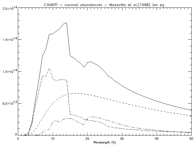
6.2 Calculating continuum intensities
For example, to calculate the free-free, free-bound and
two-photon continuum
at a temperature of 5 × 10⁶ K,
for wavelengths at 1 Å intervals between 1 and 50 Å:
freefree,5.e+6,findgen(50)+1.,ff
freebound,5.e+6,findgen(50)+1.,fb
two_photon,5.e+6,findgen(50)+1.,tp

window,0
plot,findgen(50)+1.,ff+fb+tp,xtit='Wavelength (A)'
oplot, findgen(50)+1.,ff,line=2
oplot, findgen(50)+1.,fb,line=3
oplot, findgen(50)+1.,tp,line=4
Figure 1: Continuum in the 1-50 Å range.
Note that the intensities are in units of
10−40 ergs cm3 s−1 sr−1 Å−1
per unit emission measure
∫NH Ne dh (cm−5).
If DEM values are passed to the routines
(via the keyword DEM_INT),
it is assumed that they are given as
NH Ne dh/dT . The units are
10−40 ergs cm−2 s−1 sr−1 Å−1
in this case.
6.3 Creating a synthetic spectrum with the continuum
The structure created by CH_SYNTHETIC can be restored
via CH_SS to create a spectrum.
Alternatively, it
can be used as an input to the program MAKE_CHIANTI_SPEC.
This program creates the
CHIANTI SPECTRUM structure,
an OUTPUT structure similar to the
structure created by CH_SYNTHETIC, with some additional
tags. Following the previous example:
IDL> restgen, file='ch_int_10_20_fe.genx', struct=str
IDL> make_chianti_spec, struct, lambda, struct, /CONTINUUM,$
     BIN_SIZE=0.01, instr_fwhm=0.1,  WRANGE=[10.,19.],$
      abund_name=concat_dir(concat_dir(!xuvtop,'abundance'),'cosmic.abund')
To see the contents of the structure:
IDL> help, struct,/st
IDL> help, struct.lines[0],/st
While to show the spectrum and the main contributing lines:
IDL> window,0
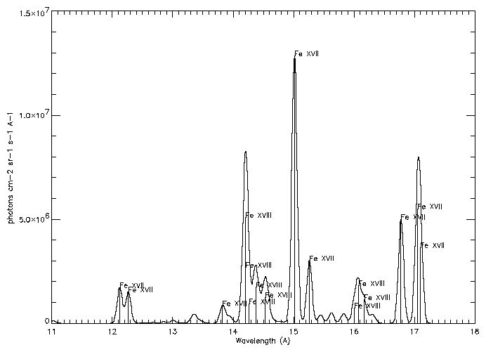
IDL> plot,struct.lambda,struct.spectrum,psym=10,xr=[11,18],/xst,$
IDL> xtit='Wavelength (A)',ytit='photons cm-2 sr-1 s-1 A-1'
IDL>    for i=0,n_elements(struct.lines) -1 do begin
IDL>      if struct.lines[i].peak gt 7e5 then begin
IDL>        xyouts, struct.lines[i].wvl,  struct.lines[i].peak, struct.lines[i].snote
IDL>        oplot,[struct.lines[i].wvl,struct.lines[i].wvl],[0,struct.lines[i].peak]
IDL>      end
IDL>    end
Figure 2: Synthetic spectrum created by MAKE_CHIANTI_SPEC.
It may be useful to save the SPECTRUM structure, that
can be later inspected with the widget CH_SS:
IDL> savegen, file='ch_spectrum_10_20_fe.genx', struct=struct
IDL> ch_write_fits, struct, 'ch_spectrum_10_20_fe.fits'
6.4 Density and temperature diagnostics from line ratios
DENS_PLOTTER and TEMP_PLOTTER are high-level widgets
for the analysis of density- and temperature-sensitive ratios of
lines from the same ion. They allow inclusion of
proton rates and photoexcitation.
The calling sequence is simple:
IDL > dens_plotter,'o_5'
to study O V.
IDL > temp_plotter,'c_4'
to study C IV.
Alternatively, you can use the command-line routines,
DENSITY_RATIOS and TEMPERATURE_RATIOS. They also allow inclusion of
proton rates and photoexcitation via KEYWORDS.
The DENSITY_RATIOS procedure
The routine DENSITY_RATIOS plots the variation of
line intensities with electron density, allowing density diagnostics
to be studied.
As an example, we can look for density sensitive
line ratios of O V in the 1000 to 1500 Å
wavelength region for densities between
108 and 1013 cm−3:
IDL >density_ratios,'o_5',1000.,1500.,8.,13.,den,rat,desc
two windows will open and plot the relative intensities of a few O V
lines. To choose the ratio of 1371.294 to 1218.393 Å line,
select first the 1371.294 Å line.
Another widget will appear to select the denominator.
Select the 1218.393 Å line.
This will chose the ratio of 1371.294 to 1218.393 which will
be plotted in a new window. Values of the density and intensity ratio will
be put into the variables den and rat and desc will contain a descriptive
string.
By specifying the keywords outfile and psfile, the ratios
values and plots will be saved in files.
The DENSITY_RATIOS procedure also allows to calculate the ratio
at user-defined value of constant temperature.
Blends are accounted for via a selection of lines.
The TEMPERATURE_RATIOS procedure
To calculate temperature sensitive line ratios of C IV for
lines between 100 and 1600 Å for temperatures between
104 and 106 K:
IDL > temperature_ratios,'c_4',100.,1600.,4.,6.,temp,rat,desc
As with density_ratios, a widget will appear that will allow you to select
the numerator. Select the 384.175 and 384.190 Å lines as these will typically
be blended in most spectrographs. Select the
1550.775 Å line
for the denominator. The ratio of (384.175
+ 384.190 Å) to the 1550.775 Å line
as a function of temperature will be plotted and
stored in the variables rat and temp, respectively.
The TEMPERATURE_RATIOS procedure also allows to calculate the ratio
at user-defined values of either constant pressure or constant density.
As with density_ratios, the outfile and psfile keywords
specify output files.
6.5 Looking at level populations
To plot the populations of the first 4 levels of Si III
as a function of density at a temperature of 3 x 10⁴ K:
IDL > plot_populations,'si_3',3.e+4,4
Optionally, output files can be created.
IDL> level_lifetime,'fe_13',4,lifetime
Level:     3s2.3p2 1S0
Lifetime (seconds):  9.098e-04
This routine calculates the lifetime of a level using the radiative
decay rates stored in the CHIANTI .wgfa file.
The 2nd input is the CHIANTI level index for the level you are
interested in (see the CHIANTI .elvlc file). The level lifetime is
returned in seconds.
IDL> metastable_levels, 'fe_13', meta
Metastable levels are:
 1 3s2.3p2 3P0
 2 3s2.3p2 3P1
 3 3s2.3p2 3P2
 4 3s2.3p2 1D2
 5 3s2.3p2 1S0
 18 3s2.3p3d 3F4
This routine returns a list of levels in an ion that are
metastable.
'meta' is an array with N elements, where N is the number of levels in
the CHIANTI ion model. It contains values of either 0 or 1, where 1
denotes that the level is metastable.
Metastable levels are identified as those for which the largest
radiative decay rate is < 105 s−1. This value can be modified by
specifying the keyword cutoff=
IDL> plot_config_energies, 'o_5'
This routine graphically displays the configuration energies for e.g. O V.
For each configuration a box is drawn whose lower and upper edges represent
the minimum and maximum energies, respectively, of the levels belonging to that configuration.
6.6 Looking at the different ionisation equilibria
If you are interested to see the differences between the
various ionisation equilibria for e.g. Mg, you can use:
IDL > plot_ioneq,'Mg'
You will be able to select one of the files, and optionally
create a postscript file of the plot.
Figure 3: Output plot of PLOT_IONEQ
6.7 Calculating contribution functions
To calculate the contribution function
( erg cm3 s−1 sr−1 by default)
vs. temperature at a specified
abundance, ionization equilibrium and pressure or density for the Fe
XXIV line at 255.1 Å:
IDL > gofnt,'fe_10',170.,180.,temperature,g,desc
temperature, g
are the arrays with the temperatures and the G(T) values.
It is possible to calculate the G(T) at either
constant electron density or pressure, via the KEYWORDS
DENSITY or PRESSURE.
The routine GOFNT allows the user to select a number
of lines. If this is done, then the total sum of the
G(T)'s of the selected lines is returned and plotted.
The KEYWORDS ABUND_NAME, IONEQ_NAME allow
to run the routine in the background, giving names of the
abundance and ionization fractions files.
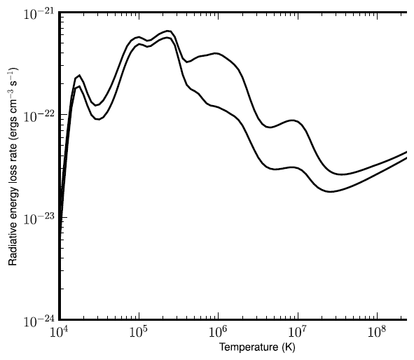
6.8 Calculating radiative losses
A procedure ('RAD_LOSS') calculates the total
radiative loss rate as a function of temperature for specified set of
abundances and/or ionization equilibria:
IDL > rad_loss,temperature,loss_rate
Figure 4: Radiative loss rate for coronal abundances (upper curve) and
photospheric abundances (lower curve).
From CHIANTI v.6, output plot of RAD_LOSS
6.9 Ionization and recombination
IDL> cross = ioniz_cross(ion,energy [, z=, ion= ])
cross is returned as the ionization cross section (cm2) as a function of the specified ion and
energy in (eV). The process of direct ionization and excitation-autoionization are both included.
For example,
cross = ioniz_cross('h_1',[14.,20.])
returns the cross section for electron collisional ionization
of H I to H II. Note that if the energies are below the ionization potential, 13.6 eV for H I, then a
cross section of zero is returned for those energies.
IDL> rate = ioniz_rate(ion, temperature [, z= , ion =])
rate is returned as the ionization rate coefficient (cm3 s−1) as a function of the specified
ion and temperature (K). The processes of direct ionization and excitation-autoionization are both
included. For example,
IDL> rate = ioniz_rate('fe_14',[1.e+6, 2.e+6])
or
IDL> rate = ioniz_rate('',[1.e+6, 2.e+6], z=26, ion=14)
returns the rate coefficient for the ionization of
Fe XIV to Fe XV at 2 temperatures.
The processes of radiative and dielectronic recombination are both included.
IDL> rate = recomb_rate(ion, temperature [,z=, ion=])
rate is returned as the recombination rate coefficient (cm3 s−1) as a function of the specified ion
and temperature (K). For example,
IDL> rate = recomb_rate('fe_14',[1.e+6, 2.e+6])
returns the rate coefficient for the recombination of Fe XIV to Fe XIII at 2 temperatures
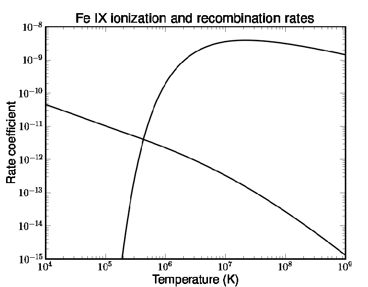
As an example, Fig 5
shows the ionization and recombination rate coefficients for Fe IX ('fe_9').
Figure 5: Ionization and recombination rate coefficients for Fe IX
IDL> make_ioneq_all, temperature, outname='new.ioneq'
a file 'new.ioneq' is created in the users working directory containing the
ionization equilibrium calculated at the specfied temperatures
for all elements from H through Zn. Users can specify a different
file name but the .ioneq extension is generally expected by the CHIANTI software.
6.10 Electron excitation rates
IDL> cc=rate_coeff('fe_13',1e6)
calculates the complete rate coefficient array for Fe XIII.
The rate coefficient is returned in units cm3 s−1.
There are 27 levels in the CHIANTI model for Fe XIII and so cc is an array of size 27 x 27.
To calculate the rate coefficient for a particular transition, do:
IDL> cc=rate_coeff('fe_13',1e6,trans=[1,20])
 Wavelength: 202.04
 Exc. rate coeff: 7.307e-09
 De-exc. rate coeff: 4.964e-09
Only the excitation rate coefficient is returned in cc. To return the
de-excitation coefficient, set trans=[20,1].
IDL> ups=spl2ups('fe_13',[1,20],1e6)
The routine spl2ups converts the spline fits stored in CHIANTI
to effective collision strengths (upsilons, as a function of temperature)
for a specified ion, transition and temperature.
In the example, 1-20 is the transition (check the .elvlc file for index
notation), and 1e6 is the temperature in Kelvin.
File translated from
TEX
by
TTH,
version 3.85.
On 27 Aug 2015, 18:47.
